These results were unable to be uploaded to fragalysis due to a 500 server error, but can be found hosted on github at the links below:
github/FoldingAtHome/covid-moonshot/master/folding-at-home_submissions/compound-set_FoldingAtHome_EE-FEP.sdf
github/FoldingAtHome/covid-moonshot/blob/master/folding-at-home_submissions/receptors.zip
Additionally, I was unable to include all the links/images I had wanted to in this post because I’m a new user. So I am leaving several in plain-text for the viewer to find and add the .com to.
Overview
Here we submit a list of 226 compounds ranked using absolute binding free energy perturbation (FEP) simulations performed on the massively parallel Folding@home distributed computing platform. Two kinds of simulations are needed for the absolute FEP: one in which a docked ligand is decoupled from the receptor, and one in which a ligand is decoupled from pure solvent.
The final score is a free energy quantity: the more negative, the better. A linear function can convert this quantity to a standard-concentration binding free energy.
Note that these 226 compounds represent a snapshot (from 05-12-2020) of data that meet our convergence criteria. We expect improved results (with a greater number converged) in the coming weeks as we continue to collect simulation data.
System Preparation
This analysis began with docked structures from John Chodera, using a procedure outlined in this post: Ensemble-hybrid-oedocking: Ensemble hybrid docking to fragment-bound Mpro structures
OpenMM and OpenForceField python modules were used to assign force-field parameters. Amber14SB was used for receptors (from Diamond Light Source), and OpenFF-1.1.0 “Parsley” (openforcefield. org/forcefields/) was used to parameterize the prospective inhibitors. Receptor-Ligand (RL) systems were created using a cubic box with solvent padding of 1.0 nm, resulting in a box length of 8.294 nm. Ligand-only (L) systems were centered in a cubic box with vectors of 3.4 nm. Systems were solvated with TIP3P water, supplemented with 100 mM NaCl counterions, minimized, and equilibrated over 10 ps to produce Gromacs 5.0.4 .gro/.top files for production.
Production on Folding@home
NVT production runs at 298.15 K were performed using GROMACS 5.0.4 on CPU clients of the Folding@home. A velocity Verlet integrator (md-vv) was used with a 4-fs timestep (made possible by artificial scaling of hydrogen masses x4). Temperature was controlled using a velocity-rescaling thermostat (v-rescale).
Free energy perturbation (FEP) was used to calculate the free energy of decoupling the ligand from the receptor, and the ligand from solvent, by sampling from a number of thermodynamic ensembles with Hamiltonians U(λcoul, λvdW) parameterized by ligand-decoupling parameters 0 ≤ λcoul, λvdW ≤ 1:
U(λcoul, λvdW) = Ubonded + (1-λcoul)Ucoul + (1-λcoul)Ucoul
The GROMACS soft-core nonbonded potentials were used (sc-alpha = 0.5, sc-power = 1, sc-sigma = 0.3) with 40 intermediate states between coupled and fully uncoupled.
github/FoldingAtHome/covid-moonshot/blob/master/folding-at-home_submissions/plots/FEP.png?raw=true
To sample from all 40 thermodynamic ensembles in a single CPU simulation, an expanded-ensemble approach was used, with protocols very similar to the work described in the most recent SAMPL blind challenge (https://www.biorxiv.org/content/10.1101/795005v1.abstract). (Huge thanks to Michael R. Shirts, who helped us figure out how to get his code to run correctly in GROMACS 5.0.4!)
To enhance sampling near the docked pose, two different harmonic restraint schemes were used. In our v2 scheme, a distance restraint using force constant k = 800.0 kJ nm-2 is placed between the alpha-carbon of MET166 and the first carbon (C1) of the ligand. In our v3 scheme, a distance restraint with the same force constant is used between the center of mass of all carbons in the ligand, and the center of mass of all alpha-carbons in hydrophobic residues (ALA, VAL, ILE, and LEU) within 1.6 nm of the ligand.
Our expanded-ensemble approach uses the Wang-Landau (WL) algorithm to perform a random walk in λ-space using a history-dependent bias potential g(λ) with metropolized-Gibbs Monte Carlo move attempts every 1 ps. Before each move attempt, the bias potential at the current λ value gets penalized by a WL increment (initially +10 kT), which serves to enhance sampling over all the λ values. Periodically, the histogram of λ sampling is assessed; if it is sufficiently “flat”, the WL increment is scaled by 0.8. Eventually, sampling over the λ values should become increasingly uniform, and the bias potential g(λ) should approach the negative of the free energy versus λ. Thus, the difference in the endpoints g(λ=0) and g(λ=1) provide an estimate of the free energy of decoupling. (NOTE: we are ignoring the harmonic restraint energy for now; we consistently find it contributes an extra +2 kT to our binding free energy estimates, and shouldn’t affect our ranks)
To collect meaningful statistics, at least five independent trajectories were initiated for each system, up to a maximum of 200 ns. In practice, only the solvated ligand simulations reach 200 ns; the receptor-ligand (RL) simulations so far typically range from 30 – 70 ns.
Analysis
Here’s an example free energy profile:
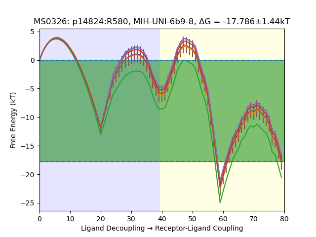
Here, the L and RL free energy profiles are shown in a continuous path, so that the vertical deviation is the predicted ∆G of binding The trajectory data used to make the above plot consists of a subset of simulations that meet our convergence criteria: a WL increment of < 0.12, predicted ∆G > 0, and standard errors < 10 kT. Additionally, only the entry with the lowest free energy prediction between both versions is included in our final results. In this case, there’s only one 45-ns RL simulation, and five 200-ns ligand-only (L) simulations. The uncertainty stems from the variance in the ligand-only simulations (which is interesting given it’s 1 µs of aggregate data)
Here’s another example:
github/FoldingAtHome/covid-moonshot/blob/master/folding-at-home_submissions/plots/example_.png?raw=true
In this second example, there are three RL trajectories that meet our convergence criteria (of lengths 21, 38, and 36 ns) and five 200-ns ligand-only (L) simulations. Here, the uncertainty arises mainly from the variance in the RL decouplings.
We have found that the most significant hurdle to obtaining converged results is sampling the protein-ligand complex. Ideally, we would like the WL increment to decrease below 0.01, but we find that most calculations appear to plateau near 0.1. Even with a converged thermodynamic profile, there remain kinetic barriers to fully exploring the many poses and binding modes accessible to a ligand that is coupled and decoupled many times from a fully flexible receptor.
While our current submission includes all predictions with a WL-increment of less than 0.12, we expect that many more systems will fit this criteria in the coming weeks.
A very preliminary comparison with the recent 2020-05-10 Data Release
We examined the results of the recently released experimental data from the first set of assayed compounds. We found that, out of the 150 or so compounds for which AVG % inhibition at 20 µM was measured, 25 of these were represented in our set of sufficiently-converged FEP results.
Using a threshold of > 10% inhibition as “active” (5 compounds) and < 10% as “inactive” (20 compounds), we computed the ROC curve below. While the sample size is very small, the enrichment of active compounds is some early evidence of the value of our FEP screening.
github/FoldingAtHome/covid-moonshot/blob/master/folding-at-home_submissions/plots/ROC.png?raw=true